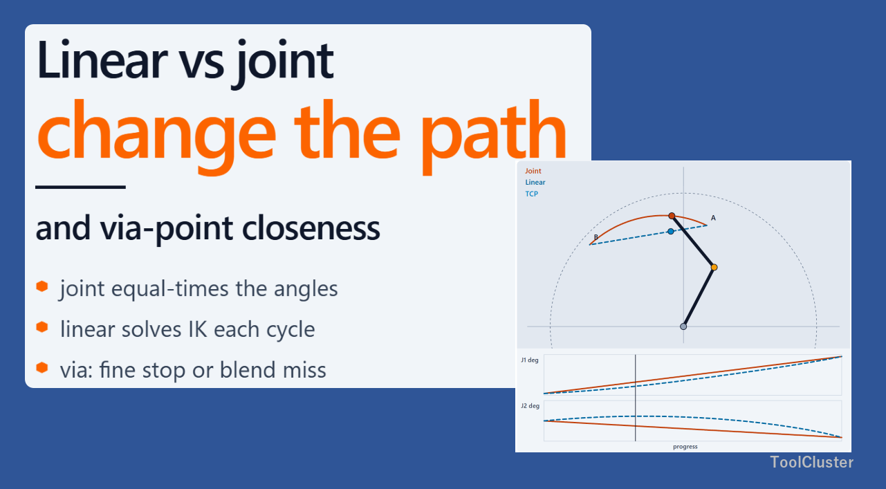
When you steer the tip of an industrial robot or a multi-axis machine, sending the tip between the same two points can still produce different paths along the way, depending on the type of command. If you move every axis through its angle in step, for example, the tool center point (TCP) traces a path closer to an arc than to the chord. A command that fills in TCP coordinates along a straight line, on the other hand, converts each intermediate point back into joint angles as it goes. So even when the arrival points look the same, the welding or sealing path in between can be a different thing entirely.
Even after you specify a straight line, the realized path can leave the commanded path depending on speed and posture. And whether the motion stops at an intermediate point with fine positioning, or passes it with blending, decides how close the TCP comes to that point. In other words, three things set the path and the closeness: the type of interpolation, speed and posture, and how via points are handled. How joints and the tip correspond in a given posture is handed to Forward and Inverse Kinematics (Part 1), the geometry of singularities to Part 2, and the lag of one servo loop to Why Servo Command and Encoder Return Drift Apart.
Key Points of This Article
| Section | The job this section places |
|---|---|
| Joint Interpolation and Linear Interpolation | Whether interpolation runs in joint angles or in TCP |
| Linear Interpolation and Inverse Kinematics | Solving the in-between points of the line every cycle |
| Path Accuracy | The same linear command, yet the realized path leaves with speed |
| Fine Positioning and Blending at Via Points | Zero speed at the point, or cutting the corner |
| Mapping onto Teaching Commands | Vendor words read only as aliases |
Joint Interpolation and Linear Interpolation
When you teach only two points, A and B, the controller fills in the commands in between on its own. That filling-in is called interpolation. And what gets decided first here is which space’s path is treated as a straight line.
Joint interpolation divides the angles so that every axis arrives at its target angle at the same instant. PTP control in the standards sits on the “specify only the points, leave the path open” side, and most teaching implements it with this joint interpolation. The TCP path is then not the chord. Even when every axis turns by an equal fraction, the tip position is a composition of the links’ trigonometric functions.
Linear interpolation, on the other hand, divides the TCP position along a straight line in the work plane. This is one kind of CP control, which does specify the path. Circular interpolation belongs to the same family, but here we look at straight lines only. Incidentally, the name tool center point refers to the point that does the work, not to the flange.
The figure below overlays the same A-to-B motion under joint interpolation and linear interpolation. Lined up under the figure are the J1 and J2 angles.
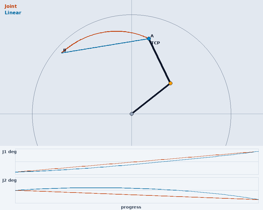
Both runs arrive at B. Along the way, though, the orange curve bows toward an arc while the blue one rides the chord. The angle traces underneath also show that keeping the TCP on the line makes the axes work at uneven rates. That is where the split comes from: joint interpolation when you want to shorten air-move time, linear interpolation when the path itself is the work. Mapping onto command names sits in a later section.
Leave the tool-tip path on in the teach-pendant preview and toggle between joint and linear interpolation; the difference shows up in a single overlay. Watching only the numbers at the arrival point, you will never see it.
Linear Interpolation and Inverse Kinematics
Riding the line means taking points along the chord as successive targets and converting each one back into joint angles. Position comes first; joints come after. That “convert back” calculation is inverse kinematics. Branch choice and elbow-up versus elbow-down stay fixed here; the details are handed to the earlier articles.
Each cycle the target TCP advances a little, and inverse kinematics issues a fresh joint command. The servo on each axis then chases that command. So linear interpolation is the job of stitching the TCP path and the joint path together every cycle. What happens when that stitching cannot keep up appears in the next section, on path accuracy.
Assuming that once a linear command is issued, the mechanism is guaranteed to run on the chord. The command specifies the commanded path; the realized path is set by joint-speed limits and posture.
Path Accuracy
The difference between the commanded path and the path the TCP actually leaves is called path accuracy. Test standards, for example, measure the same path at several speeds. On the floor the picture is the same: a slow straight line stays on the commanded path, a fast one leaves it.
One reason is joint-speed saturation. Moving along the chord at a constant tool speed makes joint angular speed swing widely with posture. Near a singularity in particular, a tiny motion of the tip calls for a large joint change. That geometry is handed to Inverse Kinematics (Part 2). Here we overlay the same linear command under slow tracking and fast tracking, and look only at the side that leaves the commanded path.
The figure below overlays the same linear command under slow tracking and fast tracking.
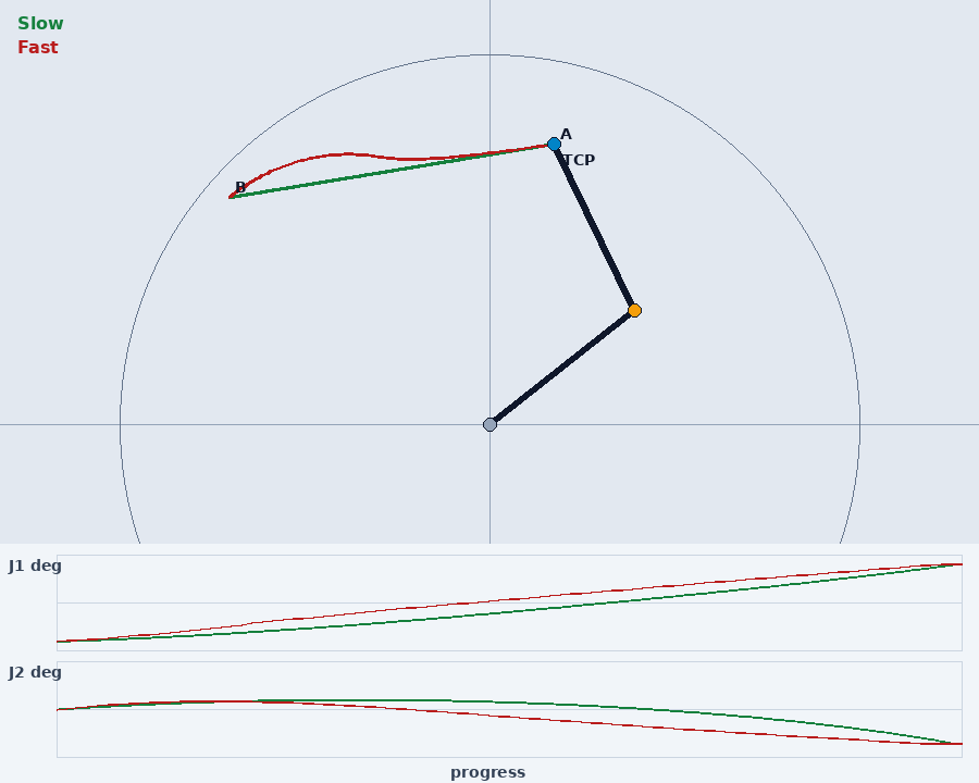
Note that the figure exaggerates the departure from the commanded path so the difference stays visible.
Raise the speed, and the required joint angular speed hits its limit. The joints then fail to reach the angles inverse kinematics asked for, and the TCP escapes to the inside or outside of the chord. This is not a fault; the command simply exceeded what the joints can deliver. The lag of one loop itself is handed to the servo command and encoder return; here we return to interpolation space and path accuracy.
Slowing only the stretches where the path matters, or moving the posture away from a singularity, comes before raising gains. Path-accuracy tests, too, are run at a fraction of rated path speed.
Fine Positioning and Blending at Via Points
When a point V is placed on the way from A to C, that V is called a via point. The question here is whether to stop at V before changing direction, or to cut nearby and pass through.
Bringing speed to zero at the point and closing the position error is fine positioning. Vendors call it fine, among other names. Blending, by contrast, keeps acceleration finite and rounds the corner into the next path; the names split again — zone, CNT, positioning level. In ISO terms the via point comes first, and fine and zone are shop-floor aliases.
The intuition for the radius that cuts the corner is an acceleration: speed squared divided by that radius. There is no need to match catalog coefficients in the formula. The faster the motion, the more the same corner is cut. So rather than memorizing “z50 means so many millimeters,” the first thing to hold is that if you do not stop, you will always miss V.
The figure below overlays the same via point V under fine positioning and blending.
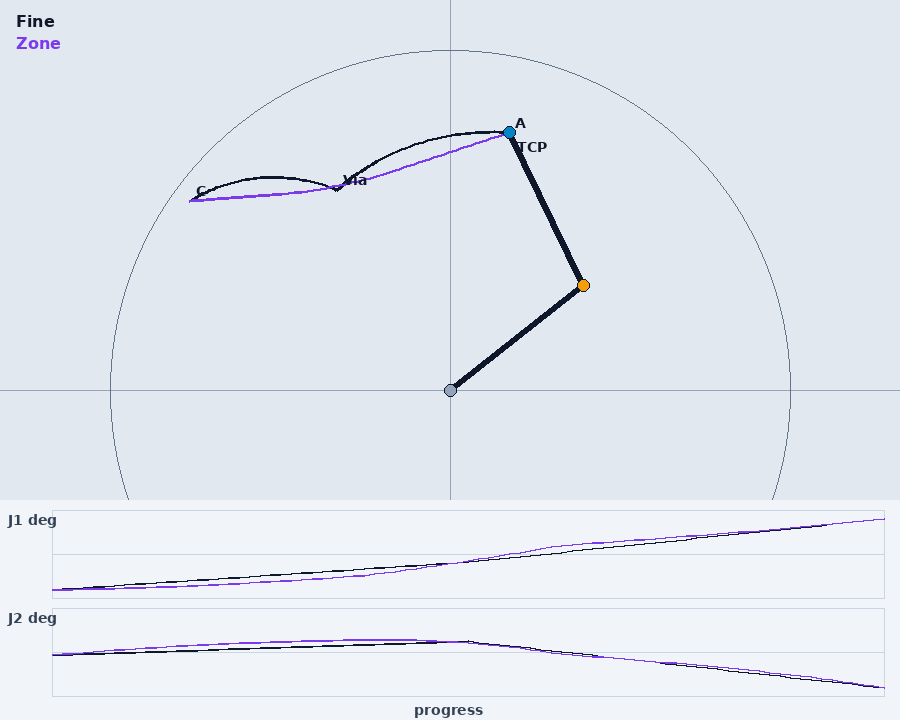
With fine positioning, the path touches V and speed drops there once. With blending, the motion enters the next path before V, and the distance to V becomes the “closeness.” So you choose by whether the sealing corner must stay sharp, or air-move time must be cut. How a cell PLC waves the path is not covered here.
Reading the blending number as the allowed distance to the point itself. Implementations also depend on speed and look-ahead. A point whose closeness must be guaranteed goes back to fine positioning.
Mapping onto Teaching Commands
The command names on the floor are aliases for the jobs so far. So this is not a cheat sheet for choosing among them; it only lays out the mapping.
| Job in this article | Common commands and parameters |
|---|---|
| Joint interpolation | MoveJ, J, MOVJ, PTP |
| Linear interpolation | MoveL, L, MOVL, LIN |
| Fine positioning | fine, FINE, positioning complete |
| Blending | zone, CNT, C_DIS, positioning level |
Circular interpolation, and interpolation that changes orientation alone, are CP of a different kind from the straight line. Orientation handling of the “position on a line, flange rotation interpolated separately” sort is also left out here.
Summary
Between the same two points, joint interpolation and linear interpolation give different TCP paths. The work of riding the line is inverse kinematics every cycle. Whether the realized path stays on the commanded path is path accuracy, and it leaves with speed. And whether the motion touches a via point or cuts past it is fine positioning versus blending.
On top of that, the command names on the floor are aliases for these jobs. MoveJ and MoveL are joint and linear interpolation; fine and zone are fine positioning and blending. Path accuracy itself has no command name; it shows up as the way a linear move drifts when you speed it up. So vendor words are not new mechanisms — read them back into this mapping and that is enough.
Frequently Asked Questions
Q1. Are joint interpolation and PTP control the same thing?
A. They relate as parent and implementation. PTP control specifies only the points and leaves the path open. In most teaching its implementation is joint interpolation, so on the floor the two overlap. Strictly, though, the definition of PTP stays on the “no path specified” side.
Q2. Is it a fault when a linear move leaves its path?
A. Usually not. Even with a straight commanded path, the realized path leaves near joint-speed limits and close to singularities. So look at speed and posture first. The one-loop lag belongs to the servo article.
Q3. Are zone or CNT numbers the distance to the point?
A. Better not to treat them as the distance itself. Blending is how a corner is cut because acceleration is finite, and it also depends on speed and look-ahead. If the TCP must touch the point, use fine positioning.
Q4. Is this article enough for the geometry of a line breaking down at a singularity?
A. No. This article looks only at the speed side of path accuracy. Full extension and solution branches belong to Inverse Kinematics (Part 2).
Q5. Is this the same phenomenon as the lag of one servo loop?
A. No, it is a separate phenomenon. The lag of one servo loop is about the command and the encoder return not lining up at the same instant. This article is about the interpolation space, and about whether the realized path stays on the commanded path. The joint servos run inside that.
Leave a Reply