Turn the joints of a robot arm by some amount and the hand ends up somewhere. Decide where you want the hand instead, and you have to work out what each joint angle should be. The first calculation is forward kinematics, the second is inverse kinematics. Together they are how you move between two ways of describing the same arm — as a set of angles, or as a point in space — and almost everything else about arms is built on top of them.
This series follows that back-and-forth on diagrams you can drag. This page covers a flat arm with two links (a planar 2R) in both directions, and then adds a third link so that the orientation of the hand can be specified as well. The shape of the region an arm can reach, and the places where its posture collapses, are the subject of part 2: workspace, singularities, and real robots.
Every figure below is a simplified model built to show a mechanism. None of them reproduces a particular manufacturer’s robot, and none includes friction, inertia, the joint limits of a real machine, or measurement noise. The “In the figure on this page” section of each part spells out what that particular figure does and does not do.
Forward kinematics (Figure 1)
How the kinematics works
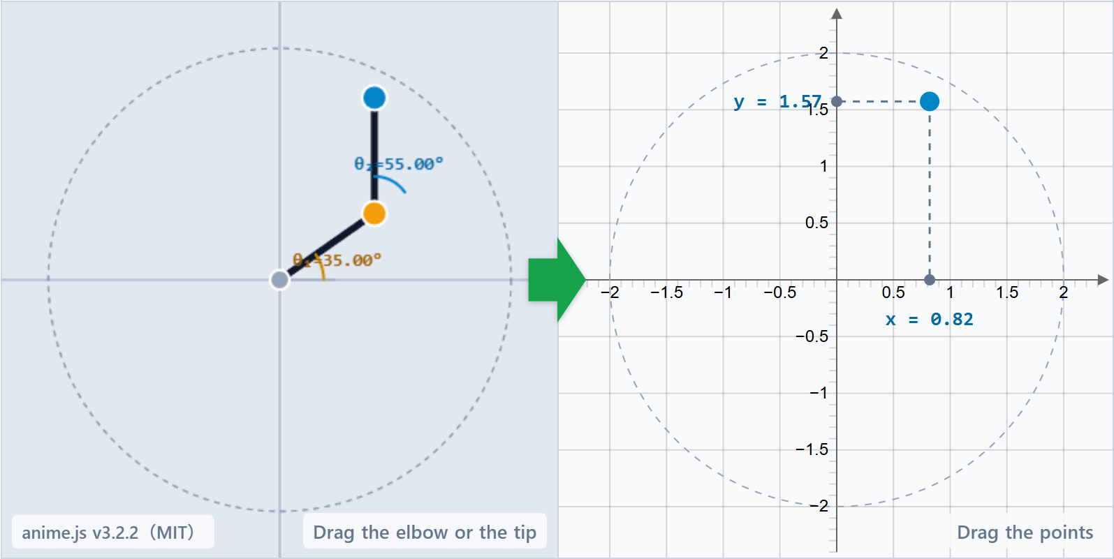
Once the joint angles θ₁ and θ₂ are fixed, the tip position (x, y) is fixed too. The first link runs from the base in the direction θ₁ for a length of L₁. The second link is bent a further θ₂ at the elbow, so it points along θ₁+θ₂, and runs for a length of L₂. Add those two vectors and you have the tip.
What matters here is that there is exactly one answer. Give the arm its angles and the hand goes to one place, with nothing to decide along the way. That obligingness belongs to the forward direction alone, as the next section shows.
In the figure on this page
The arm is on the left and the task plane, drawn as a grid, is on the right. The green arrow points from the arm to the grid: the joint angles are the cause and the tip position is the effect. The blue dots on both sides and the numbers underneath all show the same state (θ₁, θ₂, x, y), so dragging the elbow or the tip moves all three at once.
| Setup | L₁=L₂=1, base at the origin. The dashed circle is the maximum reach, L₁+L₂=2. There is no inner circle here because |L₁−L₂|=0. |
|---|---|
| Colors | Gray is the base, amber the elbow, blue the tip. The pale blue line is the path the tip has taken, shown only while Trail is on; it starts off. |
| Reading the left side | The arcs and figures are θ₁, measured from the +x axis to the first link, and θ₂, the bend at the elbow. |
| Reading the right side | The dropped perpendiculars from the tip, with x= and y= marked on the axes. |
| Controls | Drag the elbow or the tip; a draggable point spreads slightly when you hover it. Trail turns the path on and off. |
| Left out | Friction, inertia, the joint limits of a real machine, and measurement noise. |
Inverse kinematics (Figure 2)
How the kinematics works
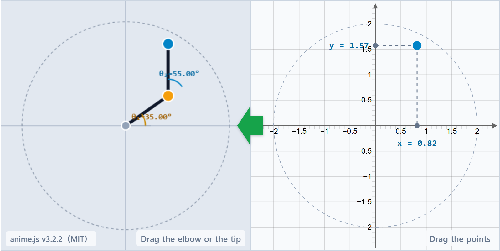
Now the position (x, y) comes first and the angles have to be worked out from it. Take the triangle whose corners are the base, the elbow and the tip. All three of its sides are known — L₁, L₂, and the distance from the base to the target — so the law of cosines gives the bend at the elbow, θ₂. With θ₂ in hand, θ₁ follows by taking the bearing of the target and subtracting the part of it the elbow accounts for.
The ± in front of the arccosine is the whole character of inverse kinematics in one symbol. In general two postures put the tip in the same place, one with the elbow raised and one with it dropped, and either will do. Where the forward direction had no choice to make, the inverse direction always comes with one attached — and on a real machine, following a path, that choice is where the difficulty starts.
In the figure on this page
The layout matches Figure 1, but the green arrow now runs the other way, from the grid to the arm. Move the tip and watch θ₁ and θ₂ being recomputed to follow it. The Elbow up and Elbow down buttons switch between the two postures while leaving the tip exactly where it is.
| Setup | Same L₁=L₂=1 as Figure 1. The tip cannot be placed outside the reach circle; drag past it and the figure pushes the tip back onto the rim. |
|---|---|
| The two solutions | Elbow up and Elbow down are the two postures that reach the same (x, y). |
| Controls | Mainly dragging the tip, though the elbow still moves. Trail turns the path on and off; it starts off. |
| Left out | Path planning, speed limits, and the details of what happens near a singularity — part 2 takes those up. |
Adding a third link (Figure 3)
How the kinematics works
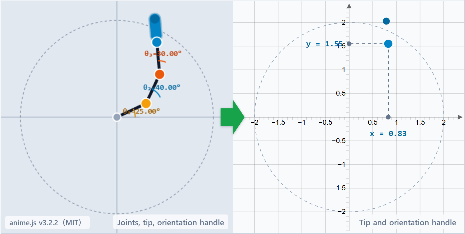
Staying in the plane and adding one more link gives a 3R arm, which can be told not only where to put the tip but also which way to face. In a plane that facing is just the sum of the joint angles, φ = θ₁+θ₂+θ₃. Setting down a part at a particular angle, or holding a tool square to a surface, is a demand of exactly this kind.
Solving the inverse problem does not mean attacking all three angles at once. It splits into three steps:
- Use φ to locate the wrist. Walk back from the tip, against the direction φ, by the length of the third link L₃, and you are at the wrist.
- Solve for that wrist (xw, yw) as a 2R problem in links 1 and 2 — which is where the elbow-up and elbow-down pair reappears.
- Fill in what is left with θ₃ = φ − θ₁ − θ₂.
In other words, pinning the orientation is what pins the wrist, and from the wrist inward you are back at Figure 2. Detaching the wrist first and solving the rest afterwards is a habit that carries over to arms working in three dimensions.
In the figure on this page
This is the smallest 3R worth drawing. The blue bar sticking out of the tip is the orientation handle, and turning it changes φ. Dragging the tip itself re-solves for position only, holding φ where it was. Read it as the 2R picture with one extra quantity to specify.
| Setup | L₁=L₂=L₃=2/3, so the maximum reach is still 2. φ = θ₁+θ₂+θ₃. |
|---|---|
| Colors | Gray is the base, yellow-amber the first joint, red-amber the second, blue the tip. The blue bar out of the tip is the orientation handle. |
| Reading the right side | Perpendiculars from the tip with x= and y=. The point at the end of the orientation handle also sets φ. |
| Controls | The handle sets φ. Dragging the tip solves for position with φ held. The second joint slides freely in the plane and the first follows it. |
| Left out | Choosing consistently among redundant solutions as the arm moves, and postures such as the roll of a six-axis wrist. |
Where six-axis industrial arms come in
How the kinematics works
The planar 2R above is the correspondence between a position (x, y) and a pair of angles (θ₁, θ₂); the planar 3R is the smallest thing that adds an orientation φ on top. An industrial six-axis arm has roughly three degrees of freedom for position and three for orientation, and with them come questions that the planar case never raises: whether a closed-form solution exists at all or the answer has to be found numerically, and which of the several valid solutions to take.
The way to read it does not change, though. Forward runs from angles to the hand, inverse from the hand back to the angles, and what grows is the number of degrees of freedom and the number of branches. The move from Figure 3 — step back to the wrist, then solve the rest as a 2R — is a pattern that keeps reappearing in three dimensions.
In this series
There is no live six-axis figure here. Both the arithmetic and the set of controls it would need belong to a different scale than the flat diagrams. What carries forward instead is the feel for 2R and 3R, and part 2 puts it to work on three questions:
- The workspace — what shape the reachable and unreachable regions actually take
- Singularities — the boundaries, such as a fully straightened arm, where the two solutions fall together and collapse
- The price of an orientation — points the arm can reach freely but can no longer reach once you also say which way to face
Summary
Forward kinematics, going from joint angles to the hand, is vector addition with a single answer. Inverse kinematics, coming back the other way, is solvable with the law of cosines and atan2, but it hands you two valid postures at once — elbow up and elbow down. One direction is obliging, the other branches; and that asymmetry is already visible in the smallest arm worth drawing.
Adding a third link buys the ability to specify orientation as well as position, and the inverse problem gains a structure: step back to the wrist, solve the 2R, fill in the remainder. That one extra quantity is enough to turn a formula into a procedure, which is the thing to notice before moving on to arms with more axes.
Part 2: workspace, singularities, and real robots takes the same planar arm and asks how far it can reach in the first place, where the two solutions collapse into one, and how much reach an imposed orientation costs.
Frequently asked questions
Q1. Does inverse kinematics always have two solutions?
A. For a planar 2R it generally does, with two exceptions. Where the arm is fully straightened — on the rim of the reach circle — θ₂ becomes 0, elbow up and elbow down are the same posture, and the two collapse into one. At the other extreme, if L₁ and L₂ are unequal and you aim very close to the base, the point is inside the hole the arm cannot reach and there are no solutions at all. Those boundaries, where the number of solutions changes, are the subject of part 2.
Q2. Why use atan2 to find θ₁?
A. Ordinary arctangent is only given the ratio y/x, so it cannot tell (x, y) from (−x, −y) and its answer can come out half a turn off. atan2 takes x and y separately and reads the quadrant from the combination of signs. An arm points in every direction, so that distinction has to be kept.
Q3. What happens if I drag the tip outside the reach circle?
A. It is pushed back onto the rim. Rather than treating an unreachable command as an error and stopping, these figures round it to the nearest reachable point. On real hardware that is a design decision: some controllers do exactly this, others reject the command outright.
Q4. In the 3R figure, why does moving the tip not change its orientation?
A. Because dragging the tip is solved as an inverse problem in position alone, with φ held fixed. To change the orientation, use the blue handle sticking out of the tip instead. Being able to command position and orientation separately is exactly what the third link bought.
Q5. Do these figures move the way a real industrial robot does?
A. No. They are simplified models that isolate the kinematic correspondence, with no friction, inertia, real joint limits, or measurement noise. A real machine has a limited range at every joint, so a posture that the arithmetic accepts may still be unreachable. Each section’s “In the figure on this page” states what that figure is not calculating.
Leave a Reply