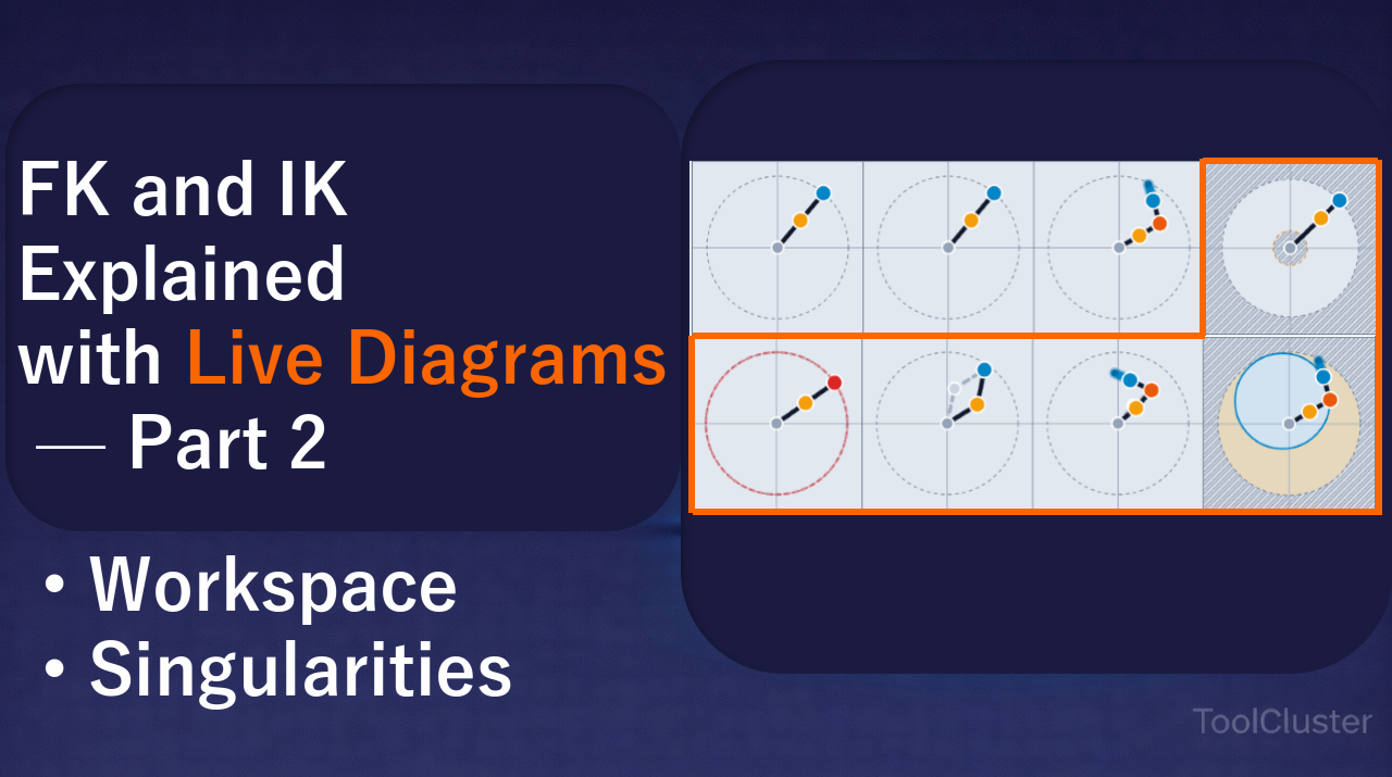
What shape is the region a robot arm can reach, and what happens at its edge? This page follows three answers on diagrams you can drag: the region a planar arm can actually get to, the singularities where its two solutions fall together and collapse, and how much of that region survives once you also insist on which way the hand is facing.
If you want the correspondence between joint angles and tip position from the beginning, start with part 1: the planar 2-link arm. Everything below reuses the notation set out there — θ₁, θ₂, θ₃ for the joints, φ for the orientation of the tip — along with the elbow-up and elbow-down pair of postures.
The workspace (Figure 1)
How the kinematics works
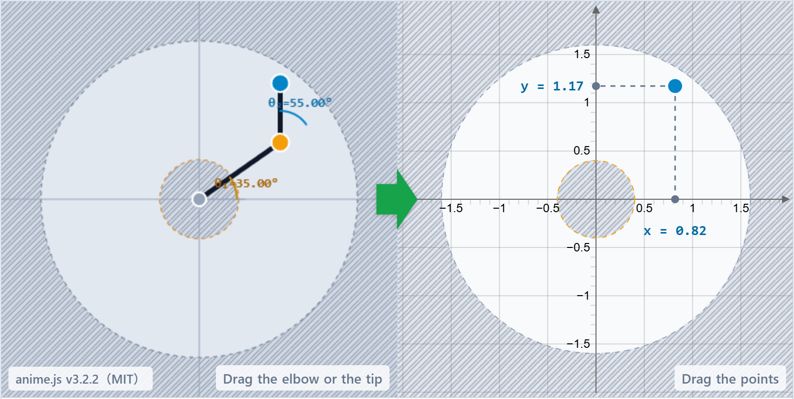
The places a planar 2R can put its tip form a ring around the base. The outer edge is the arm stretched into a straight line, at a radius of L₁+L₂. The inner edge is the second link folded all the way back over the first, at a radius of |L₁−L₂|. If the distance r from the base falls between the two the point is reachable, and if it does not, it is not.
The difference between the two link lengths is what does the work here. Make L₁ and L₂ equal and the inner radius becomes 0: the hole closes and the ring fills in to a solid disc. Make them more unequal and the unreachable hole in the middle grows, until the arm cannot pick up something sitting directly above its own base. The point of this figure is that the shape of the reachable region is settled by the dimensions of the links, not by anything the controller does.
In the figure on this page
L₁ and L₂ are on sliders. Move either one and both edges of the ring are redrawn at once, with the unreachable area filled in with hatching. The green arrow runs from the arm to the grid, because what fixes the reachable region is the dimensions of the arm rather than where you would like to put the tip.
| Setup | Planar 2R with L₁ and L₂ on sliders; they start at L₁=1, L₂=0.6 so that the inner hole is visible. Gray dashed is the maximum reach, amber dashed the minimum. |
|---|---|
| Colors | Gray is the base, amber the elbow, blue the tip. Pale blue is the trail, shown while Trail is on. The hatched area is what the arm cannot reach. |
| Reading the right side | The reachable ring and the tip’s (x, y). Drag outside the ring or into the inner hole and the tip is pushed back. |
| Controls | The L₁ and L₂ sliders, dragging the tip, Elbow up and Elbow down, and Trail; the trail starts off. |
| Left out | Obstacles, joint limits, and dynamics. The ring here is the reachable set as pure geometry. |
Near a singularity (Figure 2)
How the kinematics works
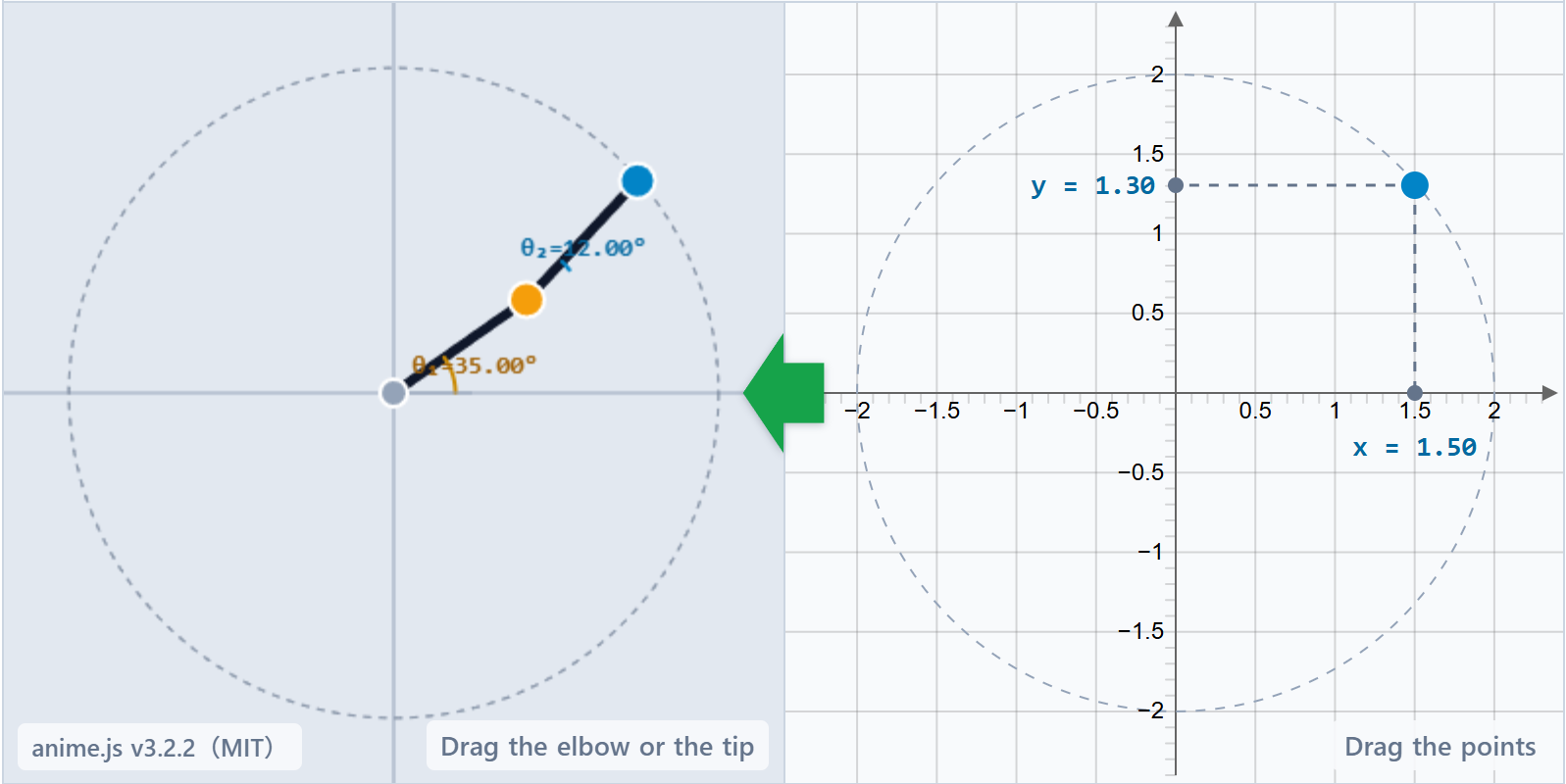
Close to the edge of the ring, a second problem appears that has nothing to do with whether a point is reachable. The matrix describing how joint motion turns into tip motion — the Jacobian — has a determinant proportional to L₁L₂ sin θ₂ for a planar 2R. When the arm is nearly straight (θ₂ near 0) or nearly folded back on itself (θ₂ near ±180°), |sin θ₂| is small and that determinant approaches zero.
That is the neighborhood of a singularity. The intuition to hold on to: it is the region where nudging the tip a small distance demands a large, fast turn of the joints. From a fully straightened posture there is nothing left to extend outward, while a small sideways move suddenly keeps the joints very busy. On real hardware this is where commanded speeds spike and a planned path falls apart.
In the figure on this page
The only indicator shown is |sin θ₂|. It is a crude stand-in for manipulability, not an evaluation of the Jacobian itself. As the value drops the tip turns red and a dashed line is drawn along the radius. Drag the tip out toward the outer circle and go looking for the red.
| Setup | L₁=L₂=1. The indicator is |sin θ₂|, a simple proxy for manipulability. |
|---|---|
| Controls | Drag the tip outward or inward. Elbow up and Elbow down, and Trail; the trail starts off. |
| Left out | Any numerical plot of the full Jacobian, and any simulation of commanded velocities. |
Where the two branches merge (Figure 3)
How the kinematics works
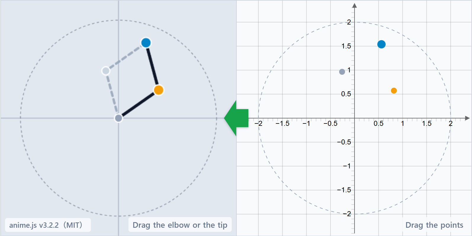
Here is the same territory approached from the other side: the fact that one tip position admits two postures, elbow up and elbow down. Move the tip out toward the outer circle and θ₂ heads for 0, which draws the two possible elbow positions steadily closer together. On the circle itself they coincide, and the two solutions have merged into one.
This is what the shrinking |sin θ₂| of Figure 2 looks like when you count solutions instead. A singularity is both a place where the posture runs out of room and a boundary where the choice of posture disappears. Read the other way round: while there is comfortable margin inside the ring, either posture is yours to use.
In the figure on this page
Both solutions are drawn at the same time, the solid one being the branch currently selected and the dashed one the alternative. The distance between the two elbows and |Δθ₂| are given as figures, so you can watch both shrink as the tip approaches the outer circle. Note that the figure only shows the two postures side by side; it does not deal with a trajectory that switches from one branch to the other while in motion.
| Setup | Planar 2R with L₁=L₂=1, showing elbow up and elbow down for one and the same (x, y). |
|---|---|
| Colors | Solid is the selected branch, dashed the other. On the right, the amber and gray points are the two elbows. |
| Controls | Dragging the tip, Elbow up and Elbow down, and Trail; the trail starts off. |
| Left out | Generating a trajectory that changes branch continuously, and enumerating the many solutions of a six-axis arm. |
The same merge with three links (Figure 4)
How the kinematics works
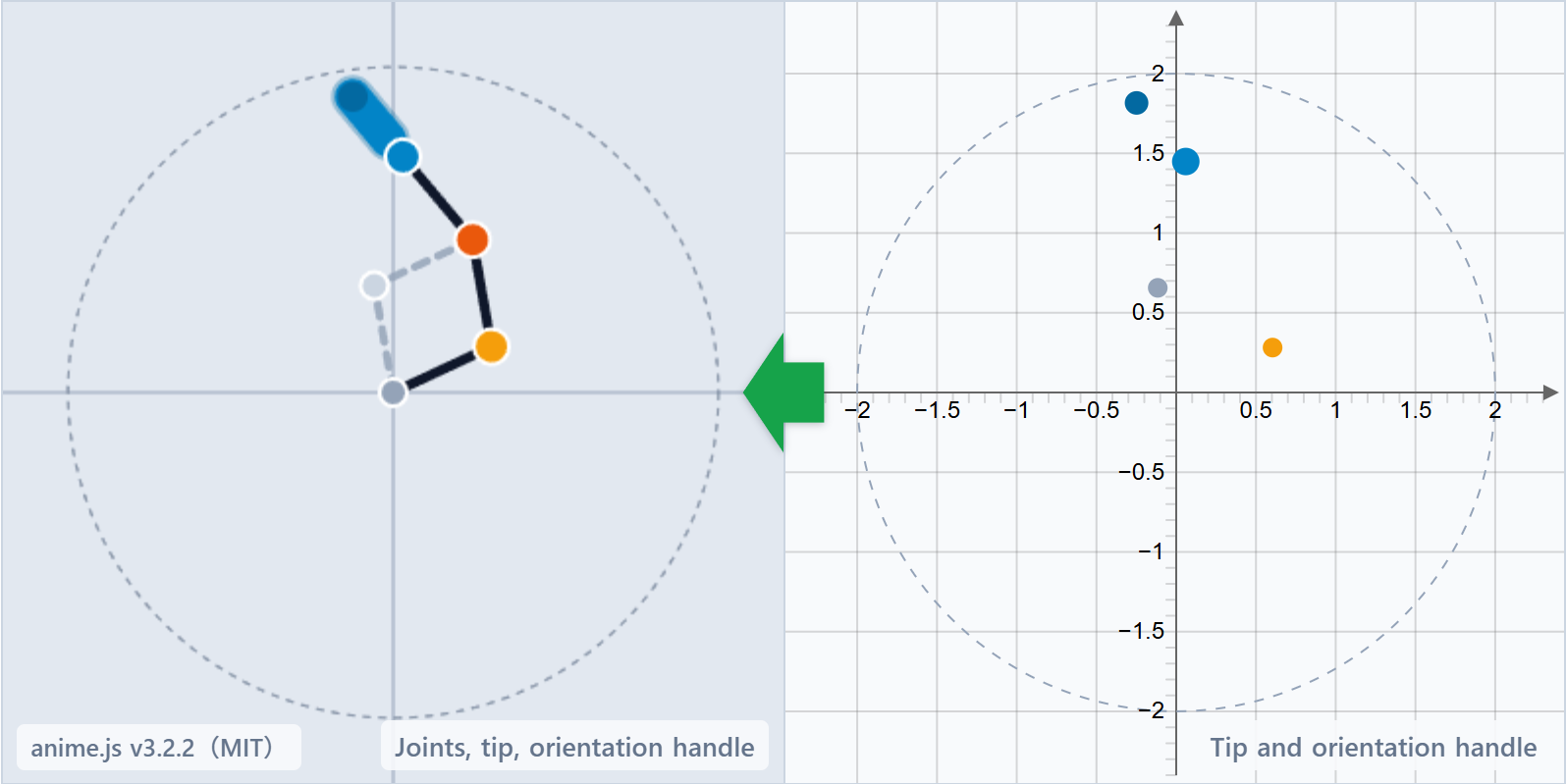
Add the third link and the same merge happens. As part 1 showed, fixing the orientation φ fixes the wrist, and what remains is a 2R inverse problem in links 1 and 2. The two-branch structure therefore survives intact, and the branches merge when that inner 2R straightens out — which is to say, when the wrist is as far from the base as it can get.
What is new is that you can move the wrist yourself. Turning the orientation handle changes φ and carries the wrist with it, so you can move between a nearly merged state and a comfortable one without touching the tip at all. More axes do not make the singular structure go away; they turn it into a question of which sub-mechanism is currently stretched out.
In the figure on this page
As in Figure 3 the two branches are solid and dashed, but what is branching now is the links 1–2 portion. Turn the orientation handle to change φ, hunt for the direction that straightens the wrist out, and the two lines close on each other. The feel this gives you — that changing the orientation changes how much room the posture has — is what Figure 5 is about.
| Setup | Planar 3R with L₁=L₂=L₃=2/3. The branching happens in links 1–2, the 2R reached through the wrist. φ is set by the orientation handle. |
|---|---|
| Controls | The orientation handle for φ, dragging the tip or the joints, and Trail. |
| Left out | Choosing consistently among redundant solutions as the arm moves, and postures such as the roll of a six-axis wrist. |
Reach once the orientation is fixed (Figure 5)
How the kinematics works
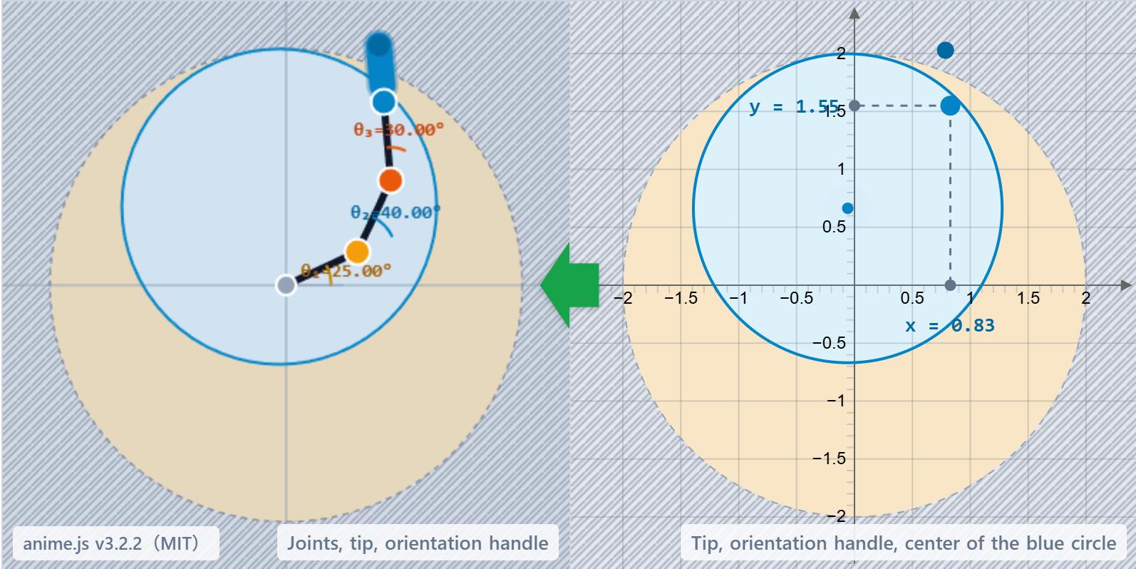
Finally, what happens to the reachable region when you specify not just where the tip goes but which way it faces. On a 3R whose three links are all of length L, ignoring orientation, the tip can be put anywhere inside a disc of radius 3L. Impose an orientation φ, though, and the wrist is pinned to the point one link-length L back from the tip against the direction φ — and that wrist has to lie within reach of links 1 and 2, inside a radius of 2L.
So the set of places the tip can go shrinks to a circle of radius 2L, centered on the point offset from the base by L in the direction φ. It is smaller than the disc of radius 3L, and as φ changes the center of it swings around. The consequence is that one and the same coordinate can be reachable at one orientation and out of reach at another. How much room is left once both the position and the orientation have to be satisfied is the entry point to what is called dexterity.
In the figure on this page
Two circles are drawn on top of each other. The gray dashed one is the outer limit when orientation is free, the blue one is what is reachable at the chosen φ, and the amber band is the difference. Move the φ slider or the orientation handle and the center of the blue circle travels around the base, taking the amber band with it. Inside that band are the points the arm could reach as a position, but cannot reach facing that way.
| Setup | Planar 3R with L₁=L₂=L₃=2/3, contrasting reach with the orientation free against reach at a chosen φ. |
|---|---|
| Controls | The orientation handle, the center of the blue circle, and the φ slider; also dragging the tip or the joints, and Trail. |
| Left out | Continuous selection among redundant trajectories, joint limits, and the full orientation of a six-axis arm. |
Where six-axis industrial arms come in
How the kinematics works
Everything above has been in a plane, but it all reappears, in a changed form, on a six-axis arm in space. The distinction between the forward and inverse directions; the reachable region being a set determined by geometry; the boundaries near a singularity where solutions collapse or multiply; the narrowing that comes with imposing an orientation. Those four are the skeleton, and the number of axes does not change them.
In this series
There is no live six-axis figure, because it is not something that can be handled with the same feel as a flat diagram. What a real six-axis arm adds is more like this:
- Degrees of freedom in orientation — in the plane, facing was the single quantity φ; in space, three rotations are involved at once.
- Choosing among solutions, continuously — the elbow-up and elbow-down split becomes many splits, and the controller has to keep choosing so that the arm does not flip branch mid-motion.
- Joint limits — an angle the arithmetic is happy with may be one the machine cannot physically turn to.
- Calibration — every discrepancy between the designed dimensions and the built ones shows up as error at the hand.
Even with all of that added, the order in which you read the problem stays the same: first check with geometry whether the point can be reached at all, then look at whether the posture has any room to work in, and only then ask whether the demanded orientation can be met.
Summary
The region a planar 2R can reach is a ring with outer radius L₁+L₂ and inner radius |L₁−L₂|. It is fixed by the dimensions of the links rather than by any skill in the control, so the only way to close the hole in the middle is to make the two links the same length. Near the edge of that ring |sin θ₂| grows small, and moving the tip a little starts to require turning the joints a lot.
Counting solutions describes the same place differently. The elbow-up and elbow-down postures draw closer as the tip approaches the outer circle, and on the circle they become one. A 3R behaves the same way: fix the orientation φ and the problem drops to a 2R reached through the wrist, so the same merge occurs. Impose φ as well, and the places the tip can go shrink from a disc of radius 3L to a circle of radius 2L, offset in the direction φ.
Reachability, room in the posture, and the demands of orientation are three things to look at in that order, and adding axes does not reorder them. For the correspondence between joint angles and tip position itself, see part 1: the planar 2-link arm.
Frequently asked questions
Q1. When does the workspace end up with a hole in the middle?
A. When the two links are of different lengths. The inner radius is |L₁−L₂|, so equal lengths give 0 and the hole disappears. Take the L₂ slider in Figure 1 and move it away from L₁, and you can watch the unreachable area around the center grow.
Q2. Are singularities something to be avoided?
A. It depends on the path you want to follow. It is not that a singularity has no solution; the property is that near one, a small movement of the tip tends to require a large movement at the joints. A fully straightened posture can also be the stiffer, more favorable one, so they are not uniformly bad. What this figure shows is the geometric fact that such a place has little margin left, and no more than that.
Q3. Can |sin θ₂| stand in for the Jacobian?
A. Only as a shortcut, and only for a planar 2R. In this particular mechanism the determinant is proportional to L₁L₂ sin θ₂, so |sin θ₂| alone tracks how close a singularity is. A general mechanism does not simplify like that and needs its singular values computed properly. This figure does not evaluate the Jacobian numerically at all.
Q4. If specifying an orientation costs reach, why specify one?
A. Because the job demands it. Inserting a part at a set attitude, or holding a tool square to a surface, is not done by getting the position right alone. The amber band in Figure 5 makes visible exactly what was given up in order to meet that demand.
Q5. Does what these figures show apply to a six-axis robot?
A. The skeleton of the reasoning carries over, but these are simplified planar models and they do not reproduce six-axis motion. Reach being determined by geometry, margin shrinking near a singularity, and an imposed orientation narrowing the region all hold for six axes too. Handling orientation in three dimensions, joint limits, and how to choose among many solutions are not in these figures.
Leave a Reply